40 Years of Alaska PFDs Adjusted for Inflation 💸 📈
Which year had the biggest PFD when adjusted for inflation?
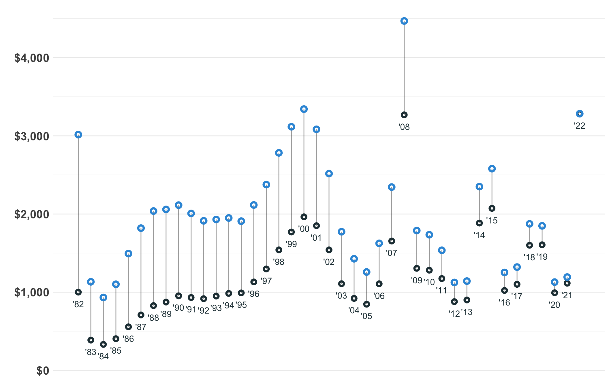
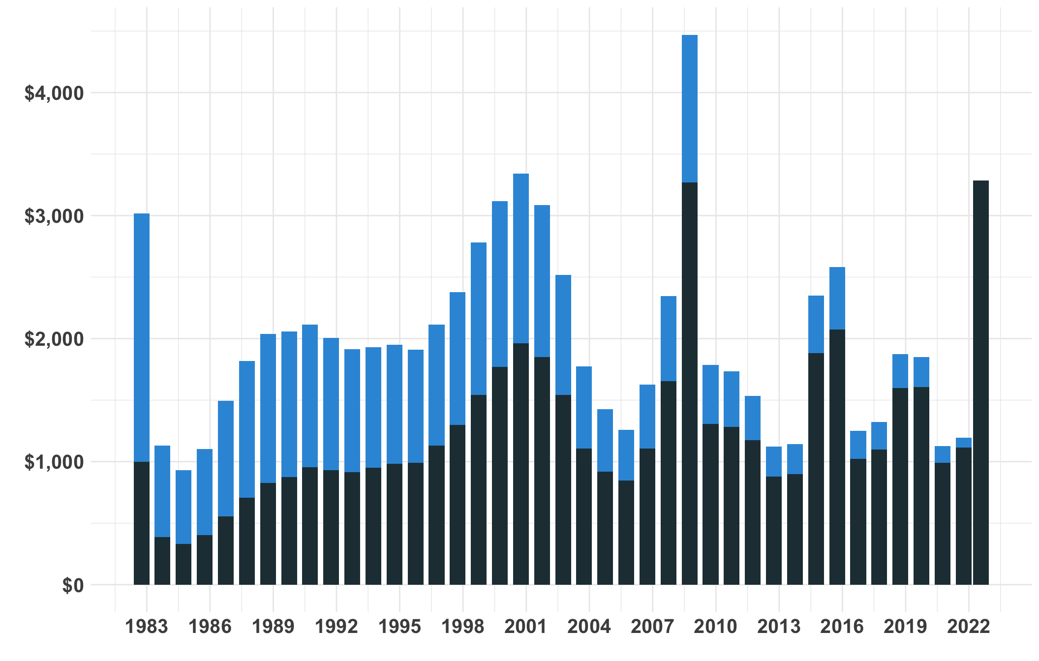
Including the energy bonus of $662, the 2022 Alaska Permanent Fund Dividend of $3,284 is the largest nominal dividend in history. But the 2008 ($4,470) and 2000 ($3,343) dividends are larger when you compare the equivalent buying power by adjusting for inflation. See the full table below.
Six dividends are worth more than $3,000 in 2022 dollars. And the first ever dividend in 1982 is almost as big as the 2022 record dividend. I include the energy bonus in 2008 and 2022 in the calculations here.
This page describes historic Alaska Permanent Fund Dividends are when adjusted for inflation. And I wanted to practice making more Quarto documents The code used to calculate the 2022 values is included at the bottom of this page.
The Consumer Price Index (CPI) used here is:
CPI for All Urban Consumers (CPI-U)
Series Title : All items in U.S. city average, all urban consumers, not seasonally adjusted Series ID : CUUR0000SA0
Seasonality : Not Seasonally Adjusted
Survey Name : CPI for All Urban Consumers (CPI-U)
Measure Data Type : All items
Area : U.S. city average
Item : All items
Downloaded 9/15/2022 from the BLS
The PFD amouts are published by the State of Alaska Dept. of Revenue.
Alaska PFDs since 1982 (+ adjusted to August 2022 dollars)
BLS CPI All Urban Consumers (CPI-U)
Alaska PFDs since 1982 (+ adjusted to August 2022 dollars)
BLS CPI All Urban Consumers (CPI-U)
Alaska PFDs since 1982 (+ adjusted to August 2022 dollars)
BLS CPI All Urban Consumers (CPI-U)
| Top Alaska PFDs in 2022 Dollars | |||
|---|---|---|---|
| Year | Nominal Dividend | Real (2022 Dollars) | Inflation $ |
| 2008 | $3,269 | $4,470 | $1,201 |
| 2000 | $1,964 | $3,343 | $1,379 |
| 2022 | $3,284 | $3,284 | $0 |
| 1999 | $1,770 | $3,116 | $1,347 |
| 2001 | $1,850 | $3,084 | $1,234 |
| 1982 | $1,000 | $3,016 | $2,016 |
| 1998 | $1,541 | $2,783 | $1,242 |
| 2015 | $2,072 | $2,580 | $508 |
| 2002 | $1,541 | $2,517 | $976 |
| 1997 | $1,297 | $2,376 | $1,080 |
| 2014 | $1,884 | $2,350 | $466 |
| 2007 | $1,654 | $2,345 | $691 |
| 1996 | $1,131 | $2,115 | $985 |
| 1990 | $953 | $2,113 | $1,161 |
| 1989 | $873 | $2,059 | $1,186 |
| 1988 | $827 | $2,038 | $1,211 |
| 1991 | $931 | $2,008 | $1,076 |
| 1994 | $984 | $1,949 | $965 |
| 1993 | $949 | $1,930 | $981 |
| 1992 | $916 | $1,913 | $997 |
| 1995 | $990 | $1,908 | $918 |
| 2018 | $1,600 | $1,874 | $274 |
| 2019 | $1,606 | $1,848 | $242 |
| 1987 | $708 | $1,819 | $1,111 |
| 2009 | $1,305 | $1,788 | $483 |
| 2003 | $1,108 | $1,773 | $666 |
| 2010 | $1,281 | $1,735 | $454 |
| 2006 | $1,107 | $1,625 | $518 |
| 2011 | $1,174 | $1,536 | $362 |
| 1986 | $556 | $1,494 | $937 |
| 2004 | $920 | $1,427 | $507 |
| 2017 | $1,100 | $1,321 | $221 |
| 2005 | $846 | $1,257 | $412 |
| 2016 | $1,022 | $1,252 | $230 |
| 2021 | $1,114 | $1,193 | $79 |
| 2013 | $900 | $1,141 | $241 |
| 1983 | $386 | $1,132 | $746 |
| 2020 | $992 | $1,128 | $136 |
| 2012 | $878 | $1,124 | $246 |
| 1985 | $404 | $1,101 | $697 |
| 1984 | $331 | $932 | $601 |
Inflation Calculation code:
Show the code
#| warning: false
#| message: false

# pfd source : https://pfd.alaska.gov/Division-Info/Summary-of-Applications-and-Payments


###CPI SOURCE: https://www.bls.gov/cpi/
# CPI for All Urban Consumers (CPI-U) 1982-84=100 (Unadjusted) - CUUR0000SA0


# pfd_raw <- read_csv("data/20210925_pfd_amounts - Sheet1.csv")

# 2022
pfd_raw <- read_csv("data/20220906_pfd_amounts.csv")


cpi_raw <- read_xlsx("data/SeriesReport-20210925161329_ebdc42.xlsx", skip=10)


##2022

# https://beta.bls.gov/dataViewer/view/timeseries/CUUR0000SA0;jsessionid=91432F7B2E9664054BA15E11CE3D4AC9

# CPI for All Urban Consumers (CPI-U)
#
# Series Title  :   All items in U.S. city average, all urban consumers, not seasonally adjusted
# Series ID :   CUUR0000SA0
# Seasonality   :   Not Seasonally Adjusted
# Survey Name   :   CPI for All Urban Consumers (CPI-U)
# Measure Data Type :   All items
# Area  :   U.S. city average
# Item  :   All items

cpi_raw <- read_xlsx("data/DataFinder-20220915202809.xlsx", skip=10) ### from


pfd <- pfd_raw %>% clean_names()


pfd <- pfd %>% select(dividend_year, dividend_amount)
pfd <- pfd %>% mutate (pfd_total = str_remove_all(dividend_amount, fixed("$")))
pfd <- pfd %>% mutate (pfd_total = str_remove_all(pfd_total, fixed(",")))
pfd <- pfd %>% mutate (pfd_total = as.numeric(pfd_total))

##############################clean up cpi######################
####################################################################
##############################3


cpi <- cpi_raw %>% clean_names()
# View(cpi)
# cpi <- cpi %>% select(year, oct, aug)
# cpi <- cpi %>% mutate(cpi_index = oct)


cpi <- cpi %>% mutate(date = ym(label))


cpi <- cpi %>% mutate (cpi_index_2022 = 296.171)

cpi <- cpi %>% mutate (cpi_ratio =  observation_value/cpi_index_2022)
cpi <- cpi %>% mutate (year = as.numeric(year))

cpi_annual <- cpi %>% filter (period == "M10" | label == "2022 Aug")


#
# cpi <- cpi %>% mutate (cpi_index = ifelse(is.na(oct), aug, oct))
# cpi <- cpi %>% mutate (cpi_index_2021 = 273.567)
# cpi <- cpi %>% mutate (cpi_ratio = cpi_index_2021/cpi_index)


pfd_cpi <- pfd %>% left_join(cpi_annual, by=c("dividend_year" = "year"))
pfd_cpi <- pfd_cpi %>% mutate (dividend_2022_dollars = dividend_amount/cpi_ratio)

# pfd_cpi <- pfd_cpi %>% mutate (pfd_amount_2021 = pfd_total*cpi_ratio)
#
# pfd_cpi1 <- pfd_cpi %>% mutate (pfd_amount_2021 = pfd_total*cpi_ratio)


##make two copoes for the plot

pfd_cpi_original <- pfd_cpi %>% mutate(time =0, pfd_amount_plot  = pfd_total)
pfd_cpi_adjusted <- pfd_cpi %>% mutate(time = 1, pfd_amount_plot = dividend_2022_dollars)


pfd_cpi <- rbind(pfd_cpi_original, pfd_cpi_adjusted)


pfd_cpi <- pfd_cpi %>% mutate (inflation_addition = dividend_2022_dollars  -pfd_total)
Line/dot chart code
Show the code
#| warning: false
#| message: false
#| fig-height: 10
#| fig-width: 11

ggplot(pfd_cpi)+
  geom_line(aes(y= dividend_year, x = pfd_amount_plot, group= dividend_year ), color="#000000", alpha=.4)+

  geom_point( data = pfd_cpi %>% filter (time ==0 ),aes(y= dividend_year, x=pfd_total ), color="#233B43", shape =21, stroke=2)+
  geom_point(data = pfd_cpi %>% filter (time ==1), aes(y= dividend_year, x=dividend_2022_dollars ), shape=21,stroke=2, size=2, color="#3498db")+
  #

  geom_text( data = pfd_cpi %>% filter (time ==0 ),aes(x= pfd_total-150, y=dividend_year, label=paste0("'",  substring(as.character(dividend_year) , 3,4)    )), color="#233B43", size=4)+
  # geom_text( data = pfd_cpi %>% filter (time ==0 ),aes(x= pfd_total-150, y=dividend_year, label= dividend_year   ), color="#233B43", size=3.4, angle=45)+
  # geom_text(data = pfd_cpi %>% filter (time ==1), aes(y= 1, x=pfd_amount_2021, label=dividend_year ), color="#3498db")+

  # ggtitle("Alaska PFD Adjusted for Inflation", "PFD amounts set to September 2022 Dollars")+
  theme_minimal()+
  # xlim(0,4400)+
  xlab("")+
  scale_y_continuous(labels = NULL, breaks = c(0,1), labs(x = ""))+
  scale_x_continuous( )+
  ylab("Year")+
      scale_x_continuous(labels=scales::dollar_format(), breaks= seq(0, 5500, by = 1000))+
   # scale_y_date( date_breaks = "4 years", date_labels = "%Y")+
  coord_flip()+
  theme(axis.text = element_text(size = 15, face="bold"))
Bar chart code:
Show the code
ggplot(pfd_cpi %>% filter(time==1))+
  # geom_col(aes(y = pfd_amount_plot , x =date, fill=time),  alpha=.9, stat="identity" )
  geom_col(aes(y = dividend_2022_dollars , x =date),fill="#3498db" , alpha=1, stat="identity" )+
    geom_col(aes(y = pfd_total , x =date), fill="#233B43",  alpha=1, stat="identity" )+
    # geom_col(aes(y = inflation_addition , x =date), fill="#233B43",  alpha=1, stat="identity" )+

  theme_minimal()+
  ylab("")+
  xlab("")+
  # xlab("")+
  # coord_flip()+
   scale_x_date( date_breaks = "3 years", date_labels = "%Y")+
    scale_y_continuous(labels=scales::dollar_format())+
    theme(axis.text = element_text(size = 15, face="bold"))


  # geom_col(aes(x=dividend_year, y = pfd_total), fill="red", alpha=.5)
Table code:
Show the code
#| warning: false
#| message: false


pfd_cpi %>% filter (time==0) %>%  arrange (desc(dividend_2022_dollars)) %>% select(-date, -cpi_index_2022, -label, -period, -pfd_total, -time, -pfd_amount_plot, -observation_value, -cpi_ratio) %>% gt() %>%
  fmt_currency(
    columns = c("dividend_amount", "dividend_2022_dollars", "inflation_addition"),
    currency = "USD",
    decimals = 0
  ) %>%
  cols_label(dividend_year = "Year",
             dividend_amount = "Nominal Dividend",
             dividend_2022_dollars = "Real (2022 Dollars)",
             inflation_addition = "Inflation $"

             ) %>%
  tab_header(title = md("**Top Alaska PFDs in 2022 Dollars**")) %>%
 tab_style(
     locations = cells_column_labels(columns = everything()),
     style     = list(
       #Give a thick border below
       cell_borders(sides =  "bottom", weight = px(3)),
       #Make text bold
       cell_text(weight = "bold")
     )
 ) %>%
     tab_options(
     #Remove border between column headers and title
     column_labels.border.top.width = px(3),
     column_labels.border.top.color = "transparent",
     #Remove border around table
     table.border.top.color = "transparent",
     table.border.bottom.color = "transparent",
     #Reduce the height of rows
     data_row.padding = px(5),
     #Adjust font sizes and alignment
     source_notes.font.size = 12,
     heading.align = "left"
   ) %>%
  data_color(columns = "dividend_2022_dollars", color = c("#7bccc4", "#08589e" )) %>%
  opt_all_caps() %>%
  opt_table_font(
    font = list(
      google_font("Chivo"),
      default_fonts()
))I like these callout boxes that come with Quarto. They are fun and cool.